class: top, left, inverse, title-slide .title[ # Analyzing Stochastic Time Series and Dynamical Systems with Topology, Stochastic Theory and Machine Learning ] .subtitle[ ## PhD Dissertation Defense ] .author[ ### <strong>Sunia Tanweer</strong> <br> — <br> Mechanical Engineering & <br> Computational Mathematics, Sciences and Engineering ] --- background-image: url("people/people.png") background-size: 1200px background-position: 100% 65% <!-- ------------------------------------------------------- --> <!-- DO NOT REMOVE --> <!-- ------------------------------------------------------- --> <!-- Adjust collaborator image size and position (DO NOT INSERT ANY CODE ABOVE THIS)--> <!-- ------------------------------------------------------- --> <!-- Adjust collaborator image size and position (DO NOT INSERT ANY CODE ABOVE THIS)--> # Acknowledgements for This Work ??? Before starting, I would like to acknowledge the funding sources, particularly AFOSR and Frontera Fellowship, and my collaborators, Firas and Narayan, who made the work in today's presentation possible. --- # Motivation ??? The motivation for my thesis stems from the growing need to develop robust methodologies for understanding and interpreting dynamic phenomena. Dynamical systems are widespread in various domains, such as aeroelasticity, chemical synthesis, neuroscience, financial markets, travel and transport, and population dynamics. My objective for this dissertation was to leverage stochsatic systems theory, machine learning and topologicla data analysis for understanding dynamical systems better. --  --  --  --  --  --  -- <br><br><br><br><br><br><br><br><br><br><br><br><br> .bg-washed-green.b--dark-green.ba.bw2.br3.shadow-1.ph1.mt1[ Objective: Leverage stochastic systems theory and topological data analysis for studying dynamical systems ] --- ??? In my comprehensive exam, I outlined several objectives I planned to achieve—at that time, Chapters 1, 3, 5, and 7 were still in progress. Since then, I’ve completed all of those targets. Let me briefly walk through what the dissertation covers. We start with a fundamental question: given a signal from a dynamical system with no clear pattern, is it stochastic or deterministically chaotic? This distinction is important because it determines the appropriate analysis tools. For stochastic systems, we focus on probability distributions, whereas for deterministic systems, the focus is on basins of attraction and attractors. So, Chapter 1 introduces a novel method for identifying whether a discrete time series arises from a stochastic or non-stochastic system. Chapter 8 presents an additional algorithm for robustly computing level crossings in discrete signals---which can be useful for the computations in the chapter 1 algorithm. Then, once a system is identified as stochastic, the next step is to characterize its underlying distribution. In Chapters 2 and 3, I develop topology-driven methods for estimation of a kernel density and for detecting changepoints or bifurcations given stochastic signals. Then, in Chapters 4 and 5 I explore applications of stochastic bifurcations in real-world systems, including aeroelastic flutter in airfoils and epidemic modeling using compartmental systems. Then, In Chapter 6, I apply topological machine learning and simplicial complex–based methods to detect bifurcations in EEG signals, with a focus on epileptic seizure classification. Finally, Chapter 7 shifts to deterministic systems, where I study the distinction between basins of attraction and attractors using a Markov chain and topological framework. Overall, this thesis aims to advance the use of topology in signal processing and dynamical systems. Due to time constraints, I will focus today on Chapters 1, 6, and 7. For the other chapters, I’ve shared short overview videos with the committee which cover the methods and results in more detail. --  --   --  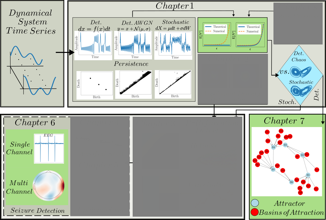 --- # Homology ??? Before we dive into each of these chapter, let's recap some basic concepts in computational topology. The shape of data is measured with something called homology. This mathematical construction returns a vector space representing some aspect of the shape. Different dimensions of homology measure different shapes – 0-dimensional homology measures the number of clusters; 1-dimensional homology measures holes or loops; 2-dimensional homology measures voids; and there are higher dimensional analogues as well. On the right are displayed the homology groups for these spaces, however all that really matters for us is the dimension of the vector space, which can be seen now As you can see, all the spaces have one connected component, so they all have 0-dimensional homology rank 1. The number of loops are measured by 1-dimensional homology. E.g, the circle here has one loop, so it has rank 1 for 1-dimensional homology. The torus has two loops, one going around the top, and one through the center, leading to a rank of 2 for 1-dim homology. -- .pull-left[ ### What is Homology? A topological invariant which assigns a vector space, `\(H_k(X)\)`, to a given topological space `\(X\)`. ### Dimension: `\(k\)` is the dimension - 0: Clusters - 1: Holes - 2: Voids ]  --   --- # Persistent Homology ??? Now we look at the modern variant of homology, known as persistent homology. This is a way to study the changing shape of a changing topological space, this filtration here, by encoding its changing homology. We keep track of when structures appear and disappear in homology, giving us information about the structure of the space itself. When a new structure appears, we say that it has taken birth, and when it disappears, we say that it has died. These birth and death pairs are recorded on a persistence diagram which we'll look at on the next few slides. -- A way to watch how the homology of a filtration (sequence) of topological spaces changes so that we can understand something about the space. -- .center[Given topological space `\(K\)` and filtration `\(K_0 \subseteq K_1 \subseteq K_2 \subseteq \cdots \subseteq K_n\)` gives a sequence of maps on homology `\(H_1(K_0) \xrightarrow{} H_1(K_1) \xrightarrow{} H_1(K_2) \xrightarrow{} \cdots \xrightarrow{} H_1(K_n)\)` ] -- .center[ Appearance `\(\xrightarrow{}\)` Birth (b) Disappearance `\(\xrightarrow{}\)` Death (d) Encoded on **Persistence Diagrams** as (b, d) ] --- # Persistence Diagram from Filtering a Simplicial Complex ??? Let's look at an example of how to construct a PD given a simplicial complex. The left side, shows the building blocks of a simplicial complex - 0 for node, 1 for edge, 2 for triangle/face and 3 for a tetrahedron. During the filtration, connected components are represented as H0 and loops are repressented as H1. So for the example simplicaial complex in the middle panel--we can vary the filtration threshold, compute the 0 and 1 homology groups, and record them on the persistence diagram displated in the right most panel. Note that the weights assigned to simplices respect a closure condition: if a face is included, the corresponding edges will be too, and if an edge is included the correspdoning nodes will be too. In practice this means that the weight of any face (e.g., a triangle) would be greater than or equal to the weights of its constituent edges, and similarly, the weight of an edge is greater than or equal to the weights of its vertices. This ensures the filtration is well-defined and consistent with the definition of a simplicial complex. So at a filtration value of 1, we see all nodes and three edges connecting four of those. At filtration value of 2, the other node combines with the rest marking the death of 4. ON the otehr hand, a loop is born due to these nodes connecting with each other. At filtration value of 4, another loop is born with the addition of this new edge. At filtration of 8, a face is added which kills the second loop while another is born. At filtration of 9, the addition of the last face causes that loop to die. Beyond this filtration, no death occurs and this connected component along with the loop always persist. So given a simplicail complex, you can filter it this way to get a persistence diagram. --  --   --   --   --   --   --   --   --- # Signal Persistence ??? For a 1D signal, the persistence can be computed similarly. Let's cover a simple example for it as well. In this case, it's easier to see the persistence diagram points as pairs of minimas and maximas of the 1D signal. E.g. in the animation, we see three persistence points taking birth when the level reaches the minimas, and dying one by one when the filtration value reaches their corresponding maximas. --  .footnote[Animation Credits: Dr Audun Myers, Pacific Northwest National Laboratory.] --- ??? Let's dive into Chapter 1 now where I discuss the problem of distinguishing stochastic signals from non-stochastic. First, I'll talk about the SOTA algos, their limitations, some mathematical background and then a new mathematical theorem which connects the persistence diagram of a signal with its pathwise or statistical characteristics. Then I show that this theorem can be used to accurately classify signals as sotchastic or non stochastic for a wide array of cases. --  --- # State of the Art ??? The current state-of-the-art includes methods like recurrence plots and Delay embeddings These are Sensitive to parameters, degrade under noise and short signals, and have a high comp cost in high dimensions Then we have methods rooted in metrics of Dynamical Systems suhc as lyapunov exponents, Correlation dimension or Entropy These typically Require a long and clean signal Then we have machine/deep learning approaches which have gotten popular in this field recently. These are limited by their generalizability. Separate models need to be trained for each system of differential equations. Finally, we have methods which use surrogate Data. These devise a Hypothesis and Compare statistics against randomized surrogates The limitations include having to generate random surrogates which can be computationally expensive along with the obvious limitation of results frequently being inconclusive leading to everyone's deep seated hatred for hypothesis testing --  --- # Function to Tree ??? Okay, so jumping into some mathematical background for this. The theorem on persistence of stochastic signals which I mentioned earlier has been derived from trees constructed from stochastic signals. So let's look at how such a tree is generated. Given a continous signal, a tree can be constructed from it by setting a root node against the global minima and maxima (shown as the red point at the bottom), from there moving upwards towards the maxima, and then adding a branch every time you hit a local minima. Each of these branches is given the length of the global maxima on the side of the branch, as shown in this animation. -- .footnote[Perez, D.: On C0-persistent homology and trees (2020). arXiv:2012.02634] <!--- `\(f: \mathbb{R} \xrightarrow{} \mathbb{R}\)` ---> <!--- `\(d_f(x,y) = f(x) + f(y) - 2\min {f(\Omega (s))}\)` ---> <!--- `\(\Omega \text{ is a path from } x \text{ to } y\)` ---> <!--- `\(T_f = \mathbb{R} / \{x \sim y \iff d_f(x, y) = 0\}\)` --->  --  --   --- # Tree to Persistence Barcode and Diagram ??? Based on this construction, you can probably intuitively tell that it has to be connected with the sublevel persistence on a signal I described earlier. Turns out, the connection is 1-to-1. Each leaf of the tree corresponds to a persistence barcode which can be used to get the the persistence diagram for that signal. That is, each branch in the tree we constructed corresponds to one point in the persistence diagram of the signal. -- .footnote[Perez, D.: On C0-persistent homology and trees (2020). arXiv:2012.02634] <!---  --->  --  --  --  --  --  --   --- # Persistence of Continuous Semimartingales ??? As I mentioned earlier, this theorem has technically been defined on trees built from stochastic signals, but since the tree and persistence diagram have a one-to-one relation, the theorem can be used to connect the persistence diagram with signal properties directly. The theorem says that the expected number of persistence points of length greater than epsilon--so basically the points which fall in this green triangle--is directly proportional to the quadratic variation, and inverse squarely proportional to epsilon in the limit of epsilon approaching zero. Since quadratic variation for a continous deterministic signal is known to be 0, this theorem would obviously not hold for deterministic signals, and should give us a reasonable way of differentiating between stochastic signals and determinstically chaotic signals by calculatnig just the quadratic variation. However, this theorem is built for continuous signlas. In reality, the signals we see aroudn us are discrete and not analog. So we can't directly use the theorem. Instead we take the followinwe yg procedure. First, we define a variable K over a range of epsilons where the number of points expected theoretically and observed computationally are nearly equal. By using a linefit, we find a region of eps where this equation holds true -- such as in the figure on the right for brownian motion. Then once we have this region of epsilons, we calculate the slope of this fitted line. For a stochastic signal, this slope should be close to a value of -2. This way we can classify if the signal is stochastic or not. -- <!--- `\(\mathbb{E}[N^\epsilon] = \frac{[M]_t}{2\epsilon^2} + \frac{2}{3} + 2\sum_{k \geq 1}(2(-1)^k - 1)\frac{\exp{\left(-\pi^2 k^2 [M]_t / 2\epsilon^2[M]_t\right)}}{\epsilon^2}\left[1 + \frac{\epsilon^2}{\pi^2 k^2 [M]_t}\right]\)` ---> .footnote[D. Perez, "On the persistent homology of almost surely c0 stochastic processes,” Journal of Applied and Computational Topology, vol. 7, pp. 879–906, July 2023.] <!--- .absolute.top-4.right-1.pa3.bg-light-gray.br3.shadow-1[$$[X]_t = \sum_{k=1}^n (X_{t_k} - X_{t_{k-1}})^2$$] ---> -- - Number of bars of length `\(\geq \epsilon\)` `\(N_\epsilon = \frac{[X]_t}{2\epsilon^2} \text{ as } \epsilon \rightarrow{} 0 \text{ where }[X]_t = \int_0^t \sigma_s^2 ds\)`  -- <br></br> > How to use this for discrete signals? <br></br> -- - `\(K(\epsilon) = \frac{N_\epsilon^{\text{emp}}}{N_\epsilon^{\text{theory}}} \approx 1 \quad \text{across small scale}\)` - `\(\log N_\epsilon \sim s \log \epsilon \text{ with } s \approx -2\)`  --- # All Systems Considered ??? For this study, I considered about 12 simulated systems falling in different categories, and some real-world financial + audio signals to test the efficiency of algorithm. These sytems range from canonical diffusions to deterministic chaotic maps/equatons and also stochastic chaos. In this presentation, I will display results from just 5 of these. --  --  --- # Example: Ornstein-Uhlenbeck ??? These first example is Ornstein uhlenbeck. OU is a classical diffusion proces - so we expect a classification of stochasticity. Each heatmap corresponds to a different signal to noise ratio. The x-axis is the discretization level of the signal, the y-axis is the length of the signal and the color displays the classification accuracy for monte carlo simulations run for these systems. Across all tested parameters, the accurayc for OU is virtually a 100%. --     .footnote[R = deterministic to stochastic ratio] --- # Example: Cox-Ingersoll-Ross ??? CIR is anotehr classical stochast proces.s Here as well, Here, across all tested parameters, the accurayc is overall high. At very low discretization of 0.01 or 0.005, we see poor classifcation perfmance. Beyond these, the algorithm accurately classifies the signal type. --     .footnote[R = deterministic to stochastic ratio] --- # Example: Linear Congruential Generator ??? Next is the LinearCongruential Generator (LCG)---which is a notoriously difficult deterministic chaotic map. For high and moderate signal to noise ratio, the signals are robustly classified as non-stochastic. Despite their apparent irregular strcuture, their excursion statistics fail to satisfy the inverse square scaling law, reflecting the absence of finite quadratic variation in the continuous–time limit. When high additive noise is introduced as for SNR 15, the system displays sharp transitions from deterministic-like to diffusion-like classification -- leading to the errors. Interestingly, for chaotic maps, the accuracy increases as discreizatoin and signal length decrease instead of the other way around. --     .footnote[SNR = signal to noise ratio] --- # Example: Lu Oscillator ??? Next is a deterministic Chaotic system, Its classification is reasonably accurate even for low SNRs of 15 and 5 (shown in middle and right panel)--granted discretization and signal length are sufficiently large. --     .footnote[SNR = signal to noise ratio] --- # Example: Stochastic Duffing ??? Finally, let's look at stochastic duffing which has both stochasticity and chaos in it. For high SNRs, the classification acc is visibly hgh. For a low signal to noise ratio, stochastic Duffing system exhibits an increase in accuracy with discretization size and decrease in acc with signal length. --     .footnote[R = deterministic to stochastic ratio] --- # Example: Audio Sounds (ESC-50 Dataset) ??? Finally, I tested the algorithm on real-world audio from the ESC-50 dataset, which contains 2000 environmental recordings spanning animal sounds, natural soundscapes, and urban noises. Since the dataset is not labeled in terms of stochastic vs. deterministic behavior, there is no ground truth available. So rather than evaluating accuracy, this experiment serves as a qualitative sanity check based on known signal characteristics. -- <br></br> | Animals | Natural soundscapes & water sounds | Human, non-speech sounds | Interior/domestic sounds | Exterior/urban noises | | :--- | :--- | :--- | :--- | :--- | | Dog | Rain | Crying baby | Door knock | Helicopter | | Rooster | Sea waves | Sneezing | Mouse click | Chainsaw | | Pig | Crackling fire | Clapping | Keyboard typing | Siren | | Cow | Crickets | Breathing | Door, wood creaks | Car horn | | Frog | Chirping birds | Coughing | Can opening | Engine | | Cat | Water drops | Footsteps | Washing machine | Train | | Hen | Wind | Laughing | Vacuum cleaner | Church bells | | Insects (flying) | Pouring water | Brushing teeth | Clock alarm | Airplane | | Sheep | Toilet flush | Snoring | Clock tick | Fireworks | | Crow | Thunderstorm | Drinking, sipping | Glass breaking | Hand saw | --- # Example: Audio Sounds (ESC-50 Dataset) ??? Let's see three specific examples. Um, The people on zoom might not hear these, so apologies in advance. The first, a thunderstorm signal—dominated by broadband, irregular fluctuations—is classified as diffusive, which aligns with our expectation of stochastic structure. Next--a chainsaw signal. This was also classified as diffusive, likely due to its noisy, high-frequency components despite some underlying periodicity. In contrast, an alarm clock signal, which exhibits strong periodic and structured patterns, is classified as non-diffusive. Overall, these examples suggest that the method is capturing meaningful distinctions in signal structure, even in the absence of explicit labels. That wraps up the chapter on distinguishing stochastic from non stochastic. The preprint can be found on the link given, and the paper is under review at Chaos. -- <div style="text-align:center;"> <!-- Images (click to flip/play audio) --> <img id="img1" src="figs/thunderstorm_real.jpg" data-default="figs/thunderstorm_real.jpg" data-alt="figs/thunderstorm.png" style="width:30%; cursor:pointer; margin-right:1%;" onclick="playAudioAndSwap('audio1','img1')"> <img id="img2" src="figs/chainsaw_real.jpg" data-default="figs/chainsaw_real.jpg" data-alt="figs/chainsaw.png" style="width:30%; cursor:pointer; margin-right:1%;" onclick="playAudioAndSwap('audio2','img2')"> <img id="img3" src="figs/clock_alarm_real.png" data-default="figs/clock_alarm_real.png" data-alt="figs/clock_alarm.png" style="width:30%; cursor:pointer;" onclick="playAudioAndSwap('audio3','img3')"> </div> -- <!-- Box appears on next click using fragment --> .bg-washed-green.b--dark-green.ba.bw2.br3.shadow-1.ph2.pv1.fragment[ Preprint available at https://arxiv.org/abs/2601.06009 and under review at Chaos. ] <!-- Audio elements --> <audio id="audio1" src="figs/thunderstorm.wav"></audio> <audio id="audio2" src="figs/chainsaw.wav"></audio> <audio id="audio3" src="figs/clock_alarm.wav"></audio> <script> function playAudioAndSwap(audioId, imgId) { const audio = document.getElementById(audioId); const img = document.getElementById(imgId); // Swap to alternate image img.src = img.dataset.alt; // Restart and play audio audio.currentTime = 0; audio.play(); // Swap back to default when audio ends audio.onended = null; audio.onended = function() { img.src = img.dataset.default; }; } </script> --- ??? On to chapter 6 on eeg signal classification for epileptic seizures, While looking for a real-world problem to apply for my bifurcation detection work in chapter 2-3, I had came across the problem of epileptic seizure detection given EEG signals. Let's take a look at this work. --  --- # Detection of Epileptic Seizures from EEG Signals ??? In EEG of an epileptic patient, three types of regimes can be found. A normal/interictal phase, a preictal phase occurring right before a seizure and an ictal phase which corresponds to a seizure. Each of these regimes' dynamics differs from the other, hence there is potential for topological machine learning to be able to classify these signals. -- <br> Three types of regimes: --  <div style="position: absolute; left:15%; top:80%; background-color: #8ebf42; border-radius: 10px; padding: 1%; font-family: Helvetica"> <b>Interictal</b> </div> --  <div style="position: absolute; left:46%; top:80%; background-color: #8ebf42; border-radius: 10px; padding: 1%; font-family: Helvetica"> <b>Preictal</b> </div> --  <div style="position: absolute; left:78%; top:80%; background-color: #8ebf42; border-radius: 10px; padding: 1%; font-family: Helvetica"> <b>Ictal</b> </div> --- # Topological Machine Learning ??? I won’t go into the full details of topological machine learning here—I’ve shared a short video with the committee that covers the methodology more thoroughly, so I’ll just give a quick overview. Starting with any data—in this case, a 1D signal—we can compute its persistence diagram, which lives in a 2D space. The next question is: how do we incorporate this into a machine learning pipeline? The key step is vectorization: we transform the persistence diagram into a finite-dimensional feature vector that can be used by standard ML models. There are several ways to do this, including Betti vectors, Carlsson coordinates, persistence landscapes, template functions, and persistence images. In this work, I will just rely on Carlsson coordinates, template functions, and persistence images. --  --   --   --- ??? So--for this classification problem--we have two types of datasets: single channel datasets where the each 1d signal has been labelled ictal, preictal or interictal. These can come from simulations by using stochastic models such as the jensen-rit or through clinical data. From each 1d signal, you can simply extract topological features and train your ML models. The other type of dataset is multivariate--where your number of channels can range from 20 to more than 150. with such a data, we can take two approaches--first where we reduce the dimension to 1 channel and extract features solely from it, or second where we extract features from each channel and data fusion at the feature level to get one feature matrix. In both cases, we'll be able to train ML models for classification. A different approach to the problem is to fuse the data at the signal level. This can be done by converting your multivariate timeseries into a higher-order simplicial complex at every timestep--and then extracting features from those simplicial complexes. Let's look at the results I got from each of these methods. -- 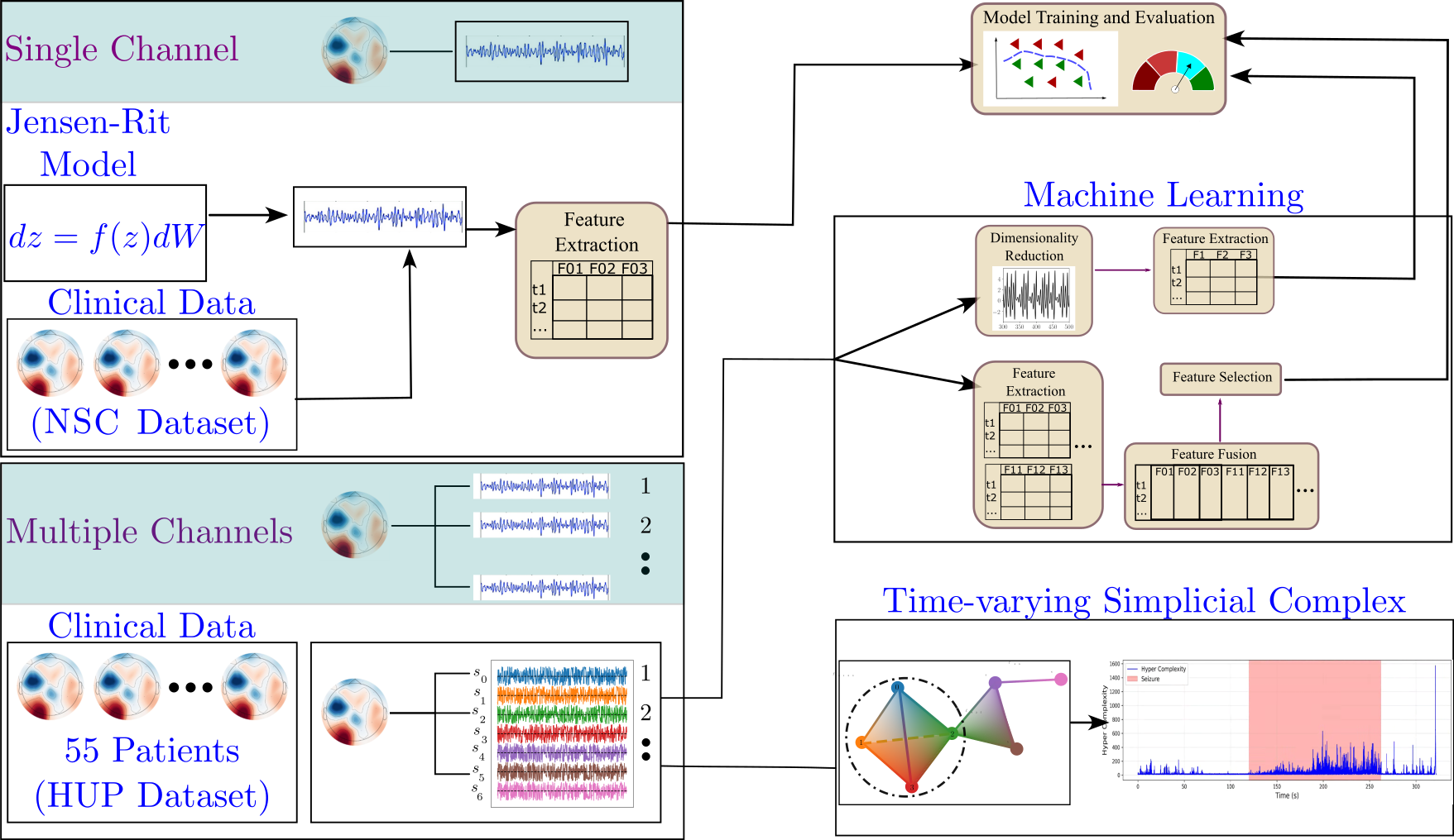 --- # Single-Channel Simulated EEG: Jansen-Rit Neural Model ??? So stage 1 of the project -- single channel simulated EEG signals from jansen rit model. The Jansen-Rit neural model is a 6 DOF system of Stochastic DEs used to simulate the interaction between pyramidal neurons and inhibitory interneurons in a brain. The difference of state variables x1 and x2 is said to simulate the behaviour of an EEG signal. Here the variable B is the bifurcation parameter changing which in the (50, 70) interval changes the EEG dynamics between precital ictal and interictal. Featurizing the persistence diagrams from these signals and training classifiers on them resulted in a 100% accuracy with simple models. -- `\(\dot{\color{green}{x_0}} = \color{green}{x_3}\)` `\(\dot{\color{green}{x_3}} = 0.06\mathcal{S}(\color{green}{x_1} - \color{green}{x_2})-0.02\color{green}{x_3}-0.01^2\color{green}{x_0}\)` `\(\dot{\color{green}{x_1}} = \color{green}{x_4}\)` `\(\dot{\color{green}{x_4}} = 0.06(\color{red}{p} + 108\mathcal{S}(135 \color{green}{x_0})) - 0.02\color{green}{x_4} - 0.01^2\color{green}{x_1}\)` `\(\dot{\color{green}{x_2}} = \color{green}{x_5}\)` `\(\dot{\color{green}{x_5}} = 0.02\color{blue}{B}(33.75\mathcal{S}(33.75 \color{green}{x_0})) - 0.04\color{green}{x_5} - 0.02^2\color{green}{x_2}\)` `\(EEG = \color{green}{x_1} - \color{green}{x_2}\)` such that `\(\mathcal{S}(z) = \frac{5}{1 + e^{0.56(6 - z)}}\)`, `\(\color{red}{p} \sim \mathcal{N}(\mu, \sigma)\)` and `\(\color{blue}{B} \in [50, 70]\)`. .bg-washed-green.b--dark-green.ba.bw2.br3.shadow-1.ph1.mt1[ 100% accuracy with classical ML models and topological features ] --- # Single-Channel Clinical EEG ??? Next I turned to a clinical dataset of 50 patients with single-channel EEG. I built classifiers with both topology and standed non-topology features used. The x-axis on the heat map represents the feature, the y-axis represents the machine learning classifier and the color-coded cells represent the test accuracy after removing any results with overfitting. The major non-TDA features used in literature are permutation entropy, renyi entropy, tsallis entropy and hurst exponents. The maximum accuracy of classification I was able to achieve using these features was 76.7% which rose to about 79% when all of them were combined. Likewise, the same analysis was conducted using TDA-based features. The maximum accuracy using these was a little over 85% with all of them combined. These models were built with no signal preprocessing and no hyperparameter tuning. -- ### Non-TDA Features 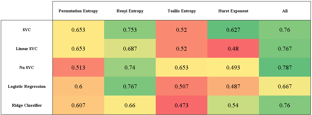 <br></br><br></br><br></br> -- ### TDA Features 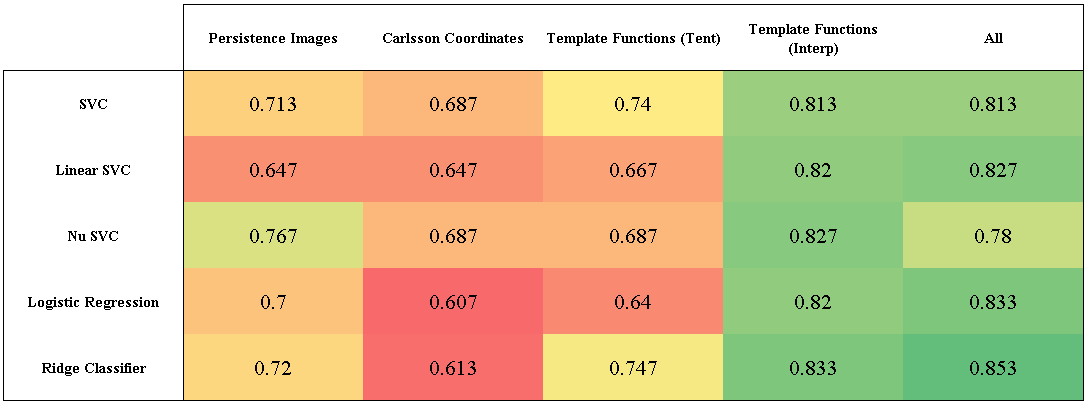 --- # Multi-Channel EEG: ML Pipeline ??? Next, I expanded this analysis to multi-channel clinical EEG data. With multi-channel EEG data, the problem lies in choosing how to combine data from all channels or how to reduce the dimensionality. I tried both approaches: first by reducing the dimension then by fusing data at the feature level. Let's look at the first one. -- 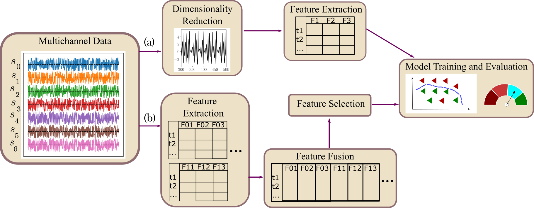 --- # Multi-Channel EEG: ML Pipeline Dimensionality Reduction  --- # Methods and Results ??? Epileptic activity is strongly linked to changes in rhythmic brain oscillations--so along with the raw EEG data, I also extracted power timeseries across standard frequency bands---alpha, beta, low gamma, high gamma, and delta. Next, I reduce dimensionality using multiple techniques like PCA or t-SNE to keep the most informative structure. Then I extracted features—both topological features, and standard entropy features for benchmarking. Finally, I fed these into classical machine learning and deep learning models to perform the three-class classification. The table lists the top 7 classification pipelines. The highest accuracy of 80% was achieved with a combination of low gamma frequency bands combined with factor analysis for dimensionality reduction with carlsson coordinates as teh features usig a convolutional network. However the accuracy with the simple classifier of logistic regression follows pretty closelt with the same featurization technique. The other top performers also use topological features, primarily carlsson coordinates, instead of the standard entropy features. <Seizures often show increased synchronization in lower frequencies like delta and theta, while abnormalities in beta and gamma can reflect disrupted cortical activity. By separating the signal into these bands, we capture physiologically meaningful patterns rather than working with noisy raw data.> --  -- <br></br><br></br><br></br><br></br><br></br> <style> table { font-size: 15px; } </style> | Rank | Accuracy | Band | Dim. Red. | Feature | Classifier | |------|----------|------------|-----------|-----------------------|---------------------| | 1 | 80.00% | Low Gamma | FA | Carlsson | Conv1DMLP | | 2 | 79.17% | Beta | FA | Carlsson | Logistic Regression | | 3 | 77.78% | Delta | LLE | Carlsson | Logistic Regression | | 4 | 77.78% | Delta | LLE | Carlsson | Linear SVC | | 5 | 77.08% | Beta | FA | Carlsson | Linear SVC | | 6 | 73.67% | Alpha | NMF | Polynomial Template | MLP (sklearn) | | 7 | 73.33% | Low Gamma | FA | Tent Template | MLP (sklearn) | --- # Accuracy Comparison ??? Performance varied across frequency bands. The delta band achieved the highest mean balanced accuracy (50.20\%), indicating that low-frequency oscillations contain useful information for seizure classification. However, the best single-performing configuration was obtained using the low gamma band (30-50 Hz), suggesting that higher frequency activity may capture seizure-related dynamics under certain model configurations. While deep learning models achieved slightly higher maximum performance, the overall performance distributions of the two model classes were similar. This result suggests that well-constructed topological feature representations can allow relatively simple models to achieve performance comparable to more complex neural network architectures. Dimensionality reduction played a critical role in classification performance. Nonlinear manifold learning techniques such as t-SNE achieved the highest mean performance across configurations, while Factor Analysis produced the best single-performing pipeline when combined with deep learning models. Linear methods such as PCA and LDA also provided stable performance across configurations. Finally, mong the evaluated topological features, polynomial based template functions achieved the highest mean performance, while Carlsson coordinates achieved the best individual result. Overall, topology-based features consistently outperformed the entropy-based baseline features, indicating that persistence can capture structural properties of EEG signals which are relevant for seizure classification. --  --  --  --  --- # Runtime Comparison ??? Alongwwith accuracies, the computational time for each feature type was computed to empirically estimate the computational complexity---for different signal lengths. Overall topological features were less computationally expensive compared to traditional entropy-based features---esp carlsson coordinates which have a sublinear runtime. --  --- # Multi-Channel EEG: ML Pipeline Feature Fusion ??? Moving onto the second pipelnie where we combine data from all channels by fusing the features extracted from all of them into one big feature matrix. A similar study was run for this comparing results by various features. Howver, the higher dimensionality created a lot of overfitting issues and led to a much smaller accuracy of about 60% compared to the dimensionality reductino pipeline. --  -- <br><br><br><br><br><br><br><br><br><br><br><br><br> .bg-washed-green.b--dark-green.ba.bw2.br3.shadow-1.ph1.mt1[ 59.5% balanced accuracy using a regularized deep multilayer perceptron classifier ] --- # Multi-Channel EEG: Co-Fluctuation Simplicial Complex ??? Finally, the thrid pipelien where we can first combine the multivariate timeseries into a simplicial complex and then extract features out of it. First, we normalize all the data. Then we convert each channgel into a separate node and give it a weight equal to its signed fluctuation computed from this formula. Likewise, edges and faces between two and three nodes resp. are given weights computed from this co-fluctuation formula as well. --  <br></br><br></br><br></br> - Normalization: `\(z_i(t) = \frac{x_i(t) - \mu_t[x_i]}{\sigma_t[x_i]}\)` - Co-Fluctuation: `\(\xi_{0\dots k}(t) = \frac{\prod_{p=0}^{k} z_p(t) - \mu_t\left[\prod_{p=0}^{k} z_p\right]}{\sigma_t\left[\prod_{p=0}^{k}z_p\right]} \quad \text{Note: } \xi_X \leq \xi_{XY} \leq \xi_{XYZ} \text{ not necessary}\)` - Weights: `\(f_{0\dots k}(t) = \text{sign}(\xi_{0\dots k}(t)) \cdot |\xi_{0\dots k}(t)| \quad \operatorname{sign}\big(\xi_{0\ldots k}(t)\big) = (-1)^{\operatorname{sgn}\left((k+1) - \left|\sum_{p=0}^{k} \operatorname{sgn}(z_p(t))\right|\right)}\)` .footnote[Andrea Santoro, et al. Higher-order organization of multivariate time series. Nature Physics, January 2023.] --- # Metrics from Persistence of Simp. Complexes ??? Once you do this for a full multicariate timeseries, you get a time-varying simplicial complex. Each of these can be filtered to get persistence diagrams from which topological metrics can be computed. For this, I am computing the time-varying betti numbers, total persistence, persistence entropy, hyper coherence and some other metrics. --  .pull-right[ - Betti Numbers - Total Persistence - Persistence Entropy - Hyper-Coherence - Hyper-Complexity - Full Coherence - Coherence Transition - Full Decoherence - Average Edge Violation ] .footnote[Andrea Santoro, Federico Battiston, Giovanni Petri, and Enrico Amico. Higher-order organization of multivariate time series. Nature Physics, January 2023.] --- # Definitions for Metrics ??? I'm going to briefly define these metrics. Once you have a weighted simplicial complex built from pairwise and three-way co-fluctuations, you can get a persistence diagram from it by filtering it--and extract the metrics mentioned earlier. If a simplex has Positive weights, it is called coherent, while a simplex with negative weights is called decoherent. To be more accurate, using the co-fluctuation formula--we don't actually get a simplicial complex. Since the cofluctuation does not have to monotonically increase with the order, we can run into the violation of the closure condition of simplicial complexs. So, for these metrics---If a triangle appears before one of its edges, that is a simplicial violation, likewise for an edge appearing before its nodes. Tehse violations are then used to commpute the hypercoherence metric as the percentage of violating coherent triangles. Then, to quantify the overall topology of the filtration, we compute persistent homology of H1 class. Its wasserstein distance from an empty persistence diagram is called hypercomplexity. We can also ask how strong the violations are using average edge violation, and we can decompose hypercomplexity into loops driven by full coherence, full decoherence, or a transition between them. Lastly, total persistence is the sum of all persistence points, while persistent entropy gives a measure of order in the persistence diagram. --  --  --- # Classification Metrics ??? Once you've these time-varying metrics, you can use each for classifying the eeg signal. On this slide, I’m showing the classification performance of these metrics we extracted from multivariate EEG signals. On the left, you can see an example topological metric time series computed from the time-varying simplicial complex for particualr patient. The shaded region corresponds to the seizure segment. What we observe is that the metric values increase and become more variable during the ictal period. We apply a simple thresholding approach using the median value of the metric to classify each time point. On the right is the ReceiverOperatingCurve curve for this same metric. This shows the trade-off between true positive rate and false positive rate across thresholds. The red point corresponds to the median threshold, which I used for reporting accuracy. The area under the curve, or AUC, gives us a threshold-independent measure of performance. At the bottom, the table summarizes results across all the topological metrics. The key takeaway is that Coherence Transition performs best, with an AUC of about 0.91 and accuracy with median threshold at around 0.77. Several other metrics—like Total Persistence and Hyper Complexity—also show reasonable discriminative power, while others are closer to random chance. Overall, this suggests that certain topological summaries of EEG dynamics carry strong information for distinguishing ictal from non-ictal states, even with a simple per-time-step classification strategy. --  -- <br></br><br></br><br></br> | Metric | Mean AUC (± std) | Mean Accuracy (± std) | |--------------------------|------------------|----------------------| | **Coherence Transition** | **0.914 ± 0.098** | **0.771 ± 0.083** | | Total Persistence | 0.770 ± 0.148 | 0.636 ± 0.097 | | Hyper Complexity | 0.765 ± 0.147 | 0.634 ± 0.096 | | Full Decoherence | 0.737 ± 0.141 | 0.619 ± 0.092 | | Hyper Coherence | 0.592 ± 0.147 | 0.553 ± 0.098 | | Full Coherence | 0.586 ± 0.139 | 0.551 ± 0.089 | | Betti # L1 norm | 0.501 ± 0.003 | 0.662 ± 0.176 | | Betti # L2 norm | 0.501 ± 0.003 | 0.662 ± 0.176 | | Avg Edge Violation | 0.452 ± 0.121 | 0.466 ± 0.080 | | Persistence Entropy | 0.380 ± 0.129 | 0.436 ± 0.086 | --- ??? That wraps up the chapter on EEG analysis. Finally, in Chapter 7, I investigate a topological approach for detecting basins of attraction in dynamical systems by utilizing hitting probabilities derived from Markov chain models of the system’s state space. --  --- # Basins of Attraction ??? The analysis of basins of attraction is fundamental in understanding the long-term behavior of nonlinear dynamical systems. These basins represent regions in the state space where trajectories converge to stable equilibria or periodic orbits. This analysis has applications in many fields. It's not always possible to do this analysis theoretically, and only numerical methods are feasible. One commonly used approach is of discretizing the phase space and computing trajectories from each grid point, However such a method can both very computationally intensive and sensitive to the discretization level. --  --  --- # State of the Art ??? The current state of the art has some limitations -- it requires maintaining the full trajectory in memory which the basin is searched. These methods also use grid discretization in a way where trajectories are snapped to the grid point. This can quicly lead to acucmulation of nuerical errors and the trajectory collapsing in systems with chaotic dynamics. The sequential nature of these methods also makes parallization difficult. Finally, the methods whcih do follow a markov chain conversion instead of a simple grid -- have relied on absoroption probabilities instead of hitting probabilities. Absorption probs can be very sensitive to noise and parameter changes rendering the anlaysis not very reliable. -- .footnote[ <div style="font-size: 0.6em; line-height: 1.1;"> (1) George Datseris, Alexandre Wagemakers; Effortless estimation of basins of attraction. Chaos 1 February 2022; 32 (2): 023104. https://doi.org/10.1063/5.0076568 (2) N. Neumann, S. Goldschmidt, and J. Wallaschek, “On the application of set-oriented numerical methods in the analysis of railway vehicle dynamics,” PAMM, vol. 4, p. 578–579, Dec. 2004. </div> ]  .pull-right[ - **Absorption probability** is the likelihood that the chain will be absorbed into a state, starting from a particular state. - **Hitting probability** is the likelihood that a particular state is reached given an initial state. ] --- # State Space to Markov Chain ??? To address these challenges, I employ a Markov chain-based model of the discretized state space, following the set-oriented numerical methodology described by Neumann et al, which turns this deterministic problem to a stochastic one, allowing me to use measures used for markov chains. For this conversion, the state space is partitioned into boxes. Each of these boxes are represented by a state in the markov chain. Then, one-step trajectories are generated from uniformaly randomly selected initial conditions inside each box. The proportions of these trajectories going from one node to another represents the transition probabilities. Having these two things completely defines a markvo chain representing the underlying deterministic system. -- .footnote[ N. Neumann, S. Goldschmidt, and J. Wallaschek, “On the application of set-oriented numerical methods in the analysis of railway vehicle dynamics,” PAMM, vol. 4, p. 578–579, Dec. 2004. </div> ]  --- # Types of Graphs ??? From this conversion, we can get multiple types of graphs. This slide shows the phase space for a vanderpol oscillator with the markov chain representaiton of it. Three types of graphs which can be computed from these are fiven in the bototm row. The first is ofcourse the markov chain's transiion matrix itself. The second is the hirring probability matrix-- which represents the likelihood that a particulat state is reached given an initla state. Both of these matrices are asymmetric graphs. To have a symmetic version, we can also transform this hitting probabilty matrix into a symmetric hitting probabililites distanfe matrix which was defined by Boyd et al in 2021. In this work, I explore the qualititative differences in the persistence diagrams from each of these three types of matrices. -- .footnote[Z. M. Boyd, N. Fraiman, J. Marzuola, P. J. Mucha, B. Osting, and J. Weare, “A metric on directed graphs and markov chains based on hitting probabilities,” SIAM Journal on Mathematics of Data Science, vol. 3, p. 467–493, Jan. 2021.]      --- # Types of Asymmetric Graph Homology ??? Since the first two types of graphs are asymmetric, I use homology theories developed specifically for directed graphs. There are four popular approaches: Dowker, flag, persistent path, and magnitude homology. This figure shows the corresponding topological summaries for a common directed graph. Each method captures different structural features, and therefore produces a different representation. One thing to note is that magnitude homology is slightly different—instead of a single filtration parameter, it is computed over two parameters. As a result, it produces a Betti matrix rather than a single persistence diagram. We’ll come back to this later in a couple of slides. --  --- # Asymmetric Graph Homology: Flag ??? The basic method of computing the filtration is the same as what we saw in the earlier slides. The building blocks are different though. E.g. in flag persistence, a 1-simplex is a directed edge not an undirected edge. a 2-simplex is an open cycle nto a closed cycle. and the same goes for a 3-simplex. So e.g. if you have a closed cycle as in the bottom image, you get a loop. But if the cycle is not closed, you get a face or a 2-simplex. -- 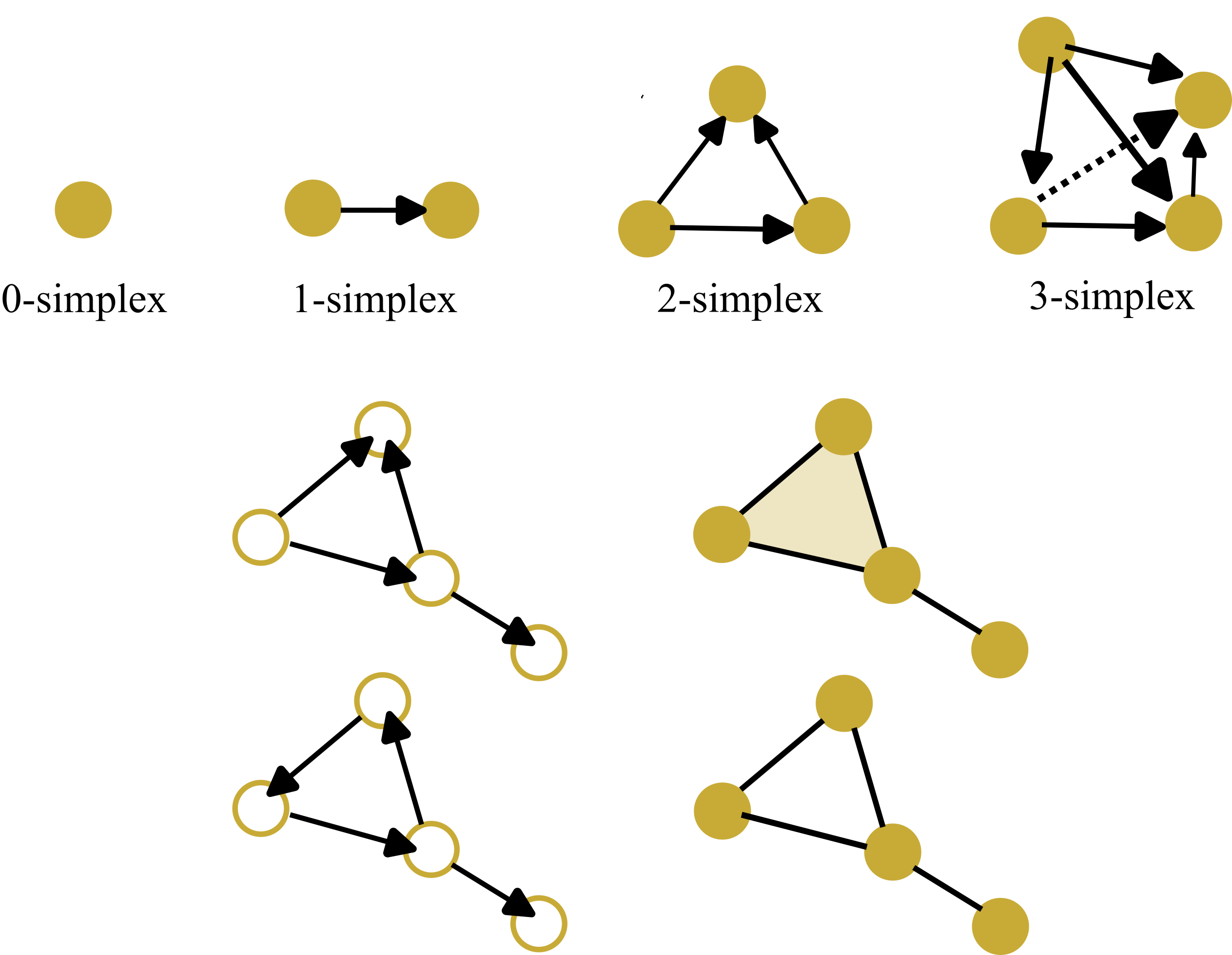 .footnote[D. Luetgehetmann, D. Govc, J. Smith, and R. Levi, “Computing persistent homology of directed flag complexes,” arXiv, 2019.] --- # Asymmetric Graph Homology: Dowker ??? Dowker complexes extract topology from binary relations between two matrices, I won' go into those details here. But once you have the graph, it gets convverted into the lawvere or the shortest path matrix. which is then filtered to get a persistence diagram simply. -- 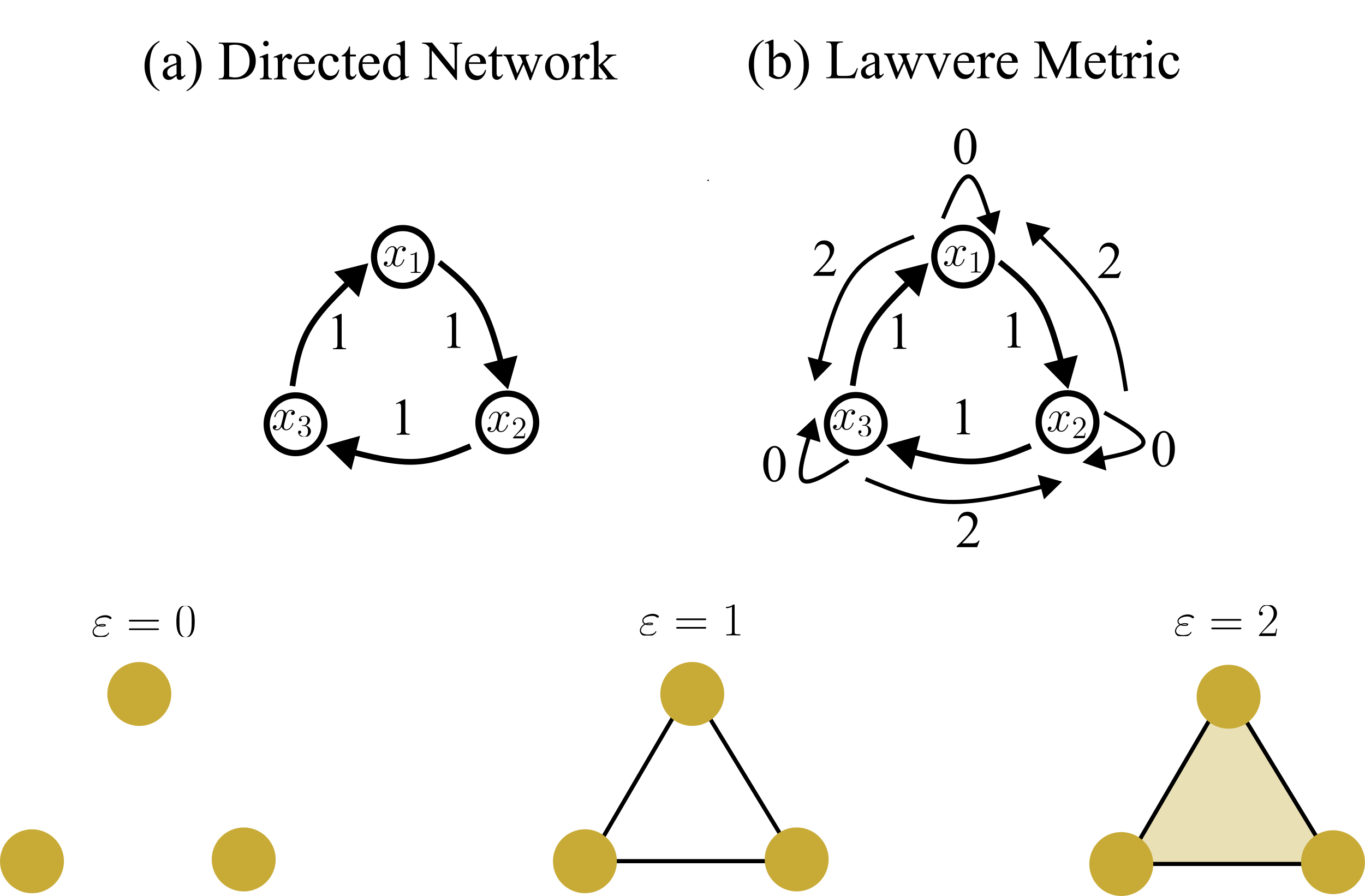 .footnote[S. Chowdhury and F. Mémoli, “A functorial dowker theorem and persistent homology of asymmetric networks,” arXiv, 2018] --- # Asymmetric Graph Homology: PPH and MH ??? Persistent path and magnitude homologies are built over paths. Given a directed graph, a `\(p\)`-path is defined as a sequence of distinct vertices such that an edge exists between each pair of consecutive vertices. So for this 6-node cycle graph. At a path length of 0, we oonly have 6 nodes and no edges. This gives an H0 count of 6 and H1 count of 0. Then at a path length of 1, we get a loop. At a path length of two, edges are added between nodes which can be connected with a distance of 2. And then, at a path length of three, edges are added between nodes which are a distance of 3 away. This leads to the loop filling in and the H1 count changes to 0. magnitude homology follows a similar procedure -- but first the graph is converted into its lawvere metric. Then since the metric has many unique path lengths, it is converted into multiple matrices with thresgoldign. And then the thresholded matrices are filtered similar to how we did it for persistent path. This then leads to a set of persistence diagrams instead of just 1. -- .footnote[ <div style="font-size: 0.6em; line-height: 1.1;"> (1) Samir Chowdhury and Facundo Mémoli. 2018. Persistent path homology of directed networks. In Proceedings of the Twenty-Ninth Annual ACM-SIAM Symposium on Discrete Algorithms (SODA '18). Society for Industrial and Applied Mathematics, USA, 1152–1169. (2) T. Leinster and M. Shulman, “Magnitude homology of enriched categories and metric spaces,” Algebraic & Geometric Topology, vol. 21, p. 2175–2221, Oct. 2021. </div> ]  -- 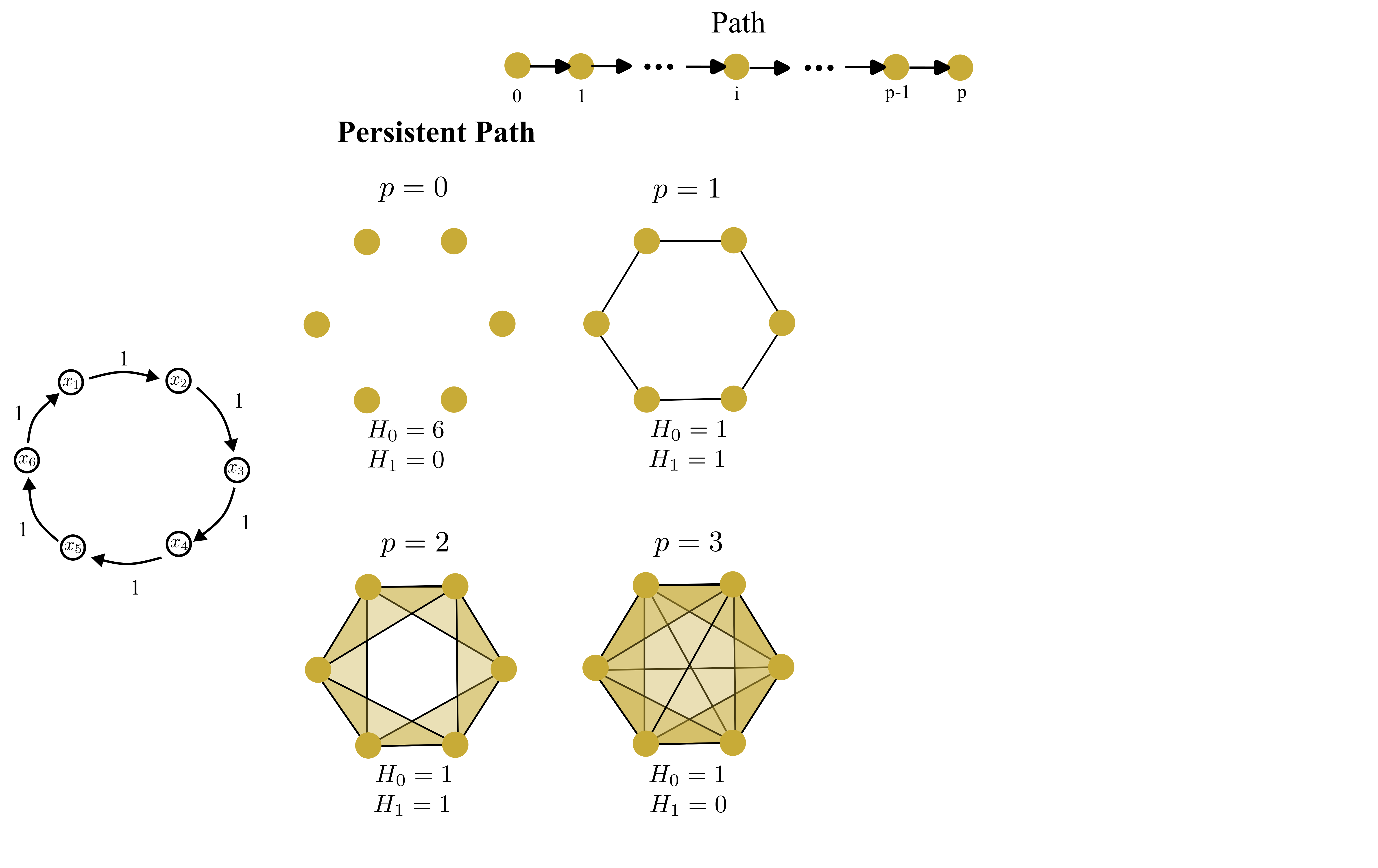 --  --- # All Systems Considered ??? That wraps up a soft intro all the different asymmetric homologies. For the study, I looked at five different systems. A fixed point in the first panel, a stable spiral shown in the second panel, a fixed radius limit cycle shown in the third panel, the duffing oscillator with two attractors shown in the fourth panel, and the vanderpol oscillator with a strong limit cycle shown in the last panel. Of these, I will display results comparing the fixed point and the vanderpol systems only. --      --- # Transition Matrix: Fixed Point vs Vanderpol ??? So, the first row shows the results for the fixed point and second row for vanderpol. The first column shows dowjer persistence, second shows flag persistence and the third one shows PPH. Results from magnitude homology were trivial throughout the study -- hence they;ve been excluded throughhout this section. For the transition matrix---dowker persistence for both fixed point and vanderpol does not show any qualitiative differencs. Flag and persistent path on the other hand do show some qualititative differnces. Flag persistence has a much higher loop count for a fixed point compared to vanderpol, while persistent path has the opposite behavriou --       --- # Hitting Probability Matrix: Fixed Point vs Vanderpol ??? For the hitting probability matrix---again dowker persistence for both fixed point and vanderpol does not show any qualitiative differencs. This time, persistent path too does not show much qualititave difference. Flag persistence on the other hand records a much higher loop count for vanderpol this time compared to the fixed point. --       --- # Hitting Probability Distance: Fixed Point vs Vanderpol ??? For the hitting probability distance matrix---flag persistence doesnot show any qualititavie differences. While dowker and persistent path have a nearly trivial persistence for the fixed point vs a non-trivial homolgoy for vanderpol oscillator. --       --- # Comparison ??? This slide summarizes the observed persistent homology features for the three graph constructions for all systems considered. The cells highlighted in green correspond to the entries where the observed persistent homology behaviour differs qualtitatively between systems with fixed point attractors and those with limit cycles attractors. Such changes suggest that these particular constructions and homologies are sensitive to differences in the underlying phase space organization---consequently they may be useful for distinguishing between basins associated with fixed points and those associated with limit cycles. [EXPAND ON EACH TABLE] While these observations are currently empirical and based on the specific examples studied here, they suggest that certain combinations of graph construction and homology computation may encode information about the type of attractor present. -- <br></br> <style> .table-container { display: flex; justify-content: space-between; gap: 20px; } .table-box { width: 32%; font-size: 12px; } table { border-collapse: collapse; width: 100%; } th, td { border: 1px solid #ccc; padding: 4px; text-align: center; } th { background: #f5f5f5; } .highlight { background-color: #d4edda; } </style> <div class="table-container"> <div class="table-box"> <b>Markov Transition Matrix (TM)</b> <table> <tr><th>System</th><th colspan="2">PPH</th><th colspan="2">Dowker</th><th colspan="2">Flag</th></tr> <tr><td></td><td>H₀</td><td>H₁</td><td>H₀</td><td>H₁</td><td>H₀</td><td>H₁</td></tr> <tr><td>Fixed Point</td><td>✓</td><td class="highlight">×</td><td>✓</td><td>✓</td><td>✓</td><td>✓</td></tr> <tr><td>Stable Spiral</td><td>✓</td><td class="highlight">×</td><td>✓</td><td>✓</td><td>0</td><td>0</td></tr> <tr><td>Limit Cycle</td><td>✓</td><td class="highlight">✓</td><td>✓</td><td>✓</td><td>0</td><td>0</td></tr> <tr><td>VdP</td><td>✓</td><td class="highlight">✓</td><td>✓</td><td>✓</td><td>0</td><td>0</td></tr> <tr><td>Duffing</td><td>✓</td><td class="highlight">✓</td><td>✓</td><td>✓</td><td>0</td><td>0</td></tr> </table> </div> <div class="table-box"> <b>Hitting Probability Distance (HPD)</b> <table> <tr><th>System</th><th colspan="2">PPH</th><th colspan="2">Dowker</th><th colspan="2">Flag</th></tr> <tr><td></td><td>H₀</td><td>H₁</td><td>H₀</td><td>H₁</td><td>H₀</td><td>H₁</td></tr> <tr><td>Fixed Point</td><td class="highlight">0</td><td>×</td><td class="highlight">0</td><td>×</td><td>✓</td><td>×</td></tr> <tr><td>Stable Spiral</td><td class="highlight">0</td><td>×</td><td class="highlight">0</td><td>×</td><td>✓</td><td>×</td></tr> <tr><td>Limit Cycle</td><td class="highlight">✓</td><td>×</td><td class="highlight">✓</td><td>×</td><td>✓</td><td>×</td></tr> <tr><td>VdP</td><td class="highlight">✓</td><td>×</td><td class="highlight">✓</td><td>×</td><td>✓</td><td>×</td></tr> <tr><td>Duffing</td><td class="highlight">✓</td><td>×</td><td class="highlight">✓</td><td>×</td><td>✓</td><td>×</td></tr> </table> </div> <div class="table-box"> <b>Hitting Probability Matrix (HPM)</b> <table> <tr><th>System</th><th colspan="2">PPH</th><th colspan="2">Dowker</th><th colspan="2">Flag</th></tr> <tr><td></td><td>H₀</td><td>H₁</td><td>H₀</td><td>H₁</td><td>H₀</td><td>H₁</td></tr> <tr><td>Fixed Point</td><td>✓</td><td>✓</td><td>✓</td><td>×</td><td>✓</td><td class="highlight">×</td></tr> <tr><td>Stable Spiral</td><td>✓</td><td>✓</td><td>✓</td><td>×</td><td>✓</td><td class="highlight">×</td></tr> <tr><td>Limit Cycle</td><td>✓</td><td>✓</td><td>✓</td><td>×</td><td>✓</td><td class="highlight">✓</td></tr> <tr><td>VdP</td><td>✓</td><td>✓</td><td>✓</td><td>×</td><td>✓</td><td class="highlight">✓</td></tr> <tr><td>Duffing</td><td>✓</td><td>✓</td><td>✓</td><td>×</td><td>✓</td><td class="highlight">✓</td></tr> </table> </div> </div> .footnote[(1) MH not shown due to trivial results throughout. (2) Cross means no significant points, tick means significant persistence points, 0 means trivial homology.] -- .bg-washed-green.b--dark-green.ba.bw2.br3.shadow-1.ph1.mt1[ Conclusion: Empirical evidence suggests certain graphs and homologies encode attractor information. ] --- # Future: Generators to Separate Attractor from Basin ??? However, just having a persistence diagram is not enough to separate the attractor from the basin. Further work, particularly involving the computation of persistence generators, will be required to determine whether these signals can reliably localize basin boundaries or identify the attractor itself. Unfortunayely, a central difficulty is that such generators are generally not unique. Even a single long lived homology class may have many valid representatives. E.g the disk on the left has a single H1 component and the two loops around it are cycle representatives for the same homology class. Similarly, the disk on the right has three H1 components and the two loops shown are possible cycle representatives. So, If persistent generators can be computed and stably interpreted for these directed filtrations, then they may provide a mechanism for differentiating between the topology of basins of attraction and the topology of the attractors themselves. --  <div style="position: absolute; left:15%; top:80%; background-color: #8ebf42; border-radius: 10px; padding: 1%; font-family: Helvetica"> <b>Phase Space</b> </div>  <div style="position: absolute; left:46%; top:80%; background-color: #8ebf42; border-radius: 10px; padding: 1%; font-family: Helvetica"> <b>Markov Chain</b> </div>  <div style="position: absolute; left:72%; top:80%; background-color: #8ebf42; border-radius: 10px; padding: 1%; font-family: Helvetica"> <b>Dowker Generator</b> </div> --   .footnote[Figure taken from Li L, Thompson C, Henselman-Petrusek G, Giusti C and Ziegelmeier L (2021) Minimal Cycle Representatives in Persistent Homology Using Linear Programming: An Empirical Study With User’s Guide. Front. Artif. Intell. 4:681117. doi: 10.3389/frai.2021.681117] --- ??? On that note, I conclude tehe technical part of my defense. The rest of the chapters can be read in the dissertation once its approved and available on proquest. --  --- # Acknowledgements ??? I would like to acknowledge all the incredible people I’ve had the privilege of collaborating with over the past four years. At MSU, I’ve also been fortunate to work with my supervisor, Dr Munch and Dr Max Chumley who graduated last year. Their influence shaped most of my dissertation. I also met some researchers through AMS' Mathematical Research Communities - and connecting with them taught me a lot about asymmetric homologies. Since May of last year, I've also been interning with the Georgia Tech Research Institute. Working there with Dr. Branden Stone gave me a window into research outside of acadaemic labs. Finally, I’m grateful to my two collaborators Dr. Mamis and Dr. Subramaniyam for bringing some interesting applications for me to test my algorithms on. Working with all of them has been a rewarding experience, and I appreciate the time, knowledge, and effort put in by everyone. --  --- <style type="text/css"> .small-text { font-size: 15px; } </style> ??? These productive collaborations led me to have a number of published papers and preprints, An NSF funded computational science fellowship to access the fastest supercomputer in the US---as well as the Fitch Beach award for outstanding doctoral research in mechanical engineering. --  --- # The End: Where Next? ??? This concludes my presentation and hopefully the journey at MSU. Granted I pass this defense, I will be joining the maths department at UMich as a reserach track faculty to establish a new intelligent algorithms core. Thank you for listening. -- - Research-Track Faculty position at MCAIM-UMich - Establish a new Algorithm Core   --- class: center, middle # Thank You! <div class="rotating-text"> <span>Questions?</span> <span>¿Preguntas?</span> <span>Fragen?</span> <span>質問はありますか？</span> <span>سوالات؟</span> <!-- Urdu --> <span>أسئلة؟</span> <!-- Arabic --> </div>